First Steps at Coffea-Casa @ UNL
Prerequisites
The primary mode of analysis with coffea-casa is coffea. Coffea provides plenty of examples to users in its documentation. Further resources, meant to run specifically on coffea-casa, can be found in the sidebar under the “Gallery of Coffea-casa Examples” section or the appropriate repository here.
Knowledge of Python is assumed. The standard environment for coffea analyses is within Jupyter Notebooks, which allow for dynamic, block-by-block execution of code. Coffea-casa employs the JupyterLab interface. JupyterLab is designed for hosting Jupyter Notebooks on the web and permits the usage of additional features within its environment, including Git access, compatibility with cluster computing tools, and much, much more.
If you aren’t familiar with any of these tools, please click on the links above and get acquainted with how they work before delving into coffea-casa.
Access
Important
For CMS or opendata files, please see the relevant sections for coffea-casa at T2 Nebraska. For ATLAS files, see coffea-casa at UChicago.
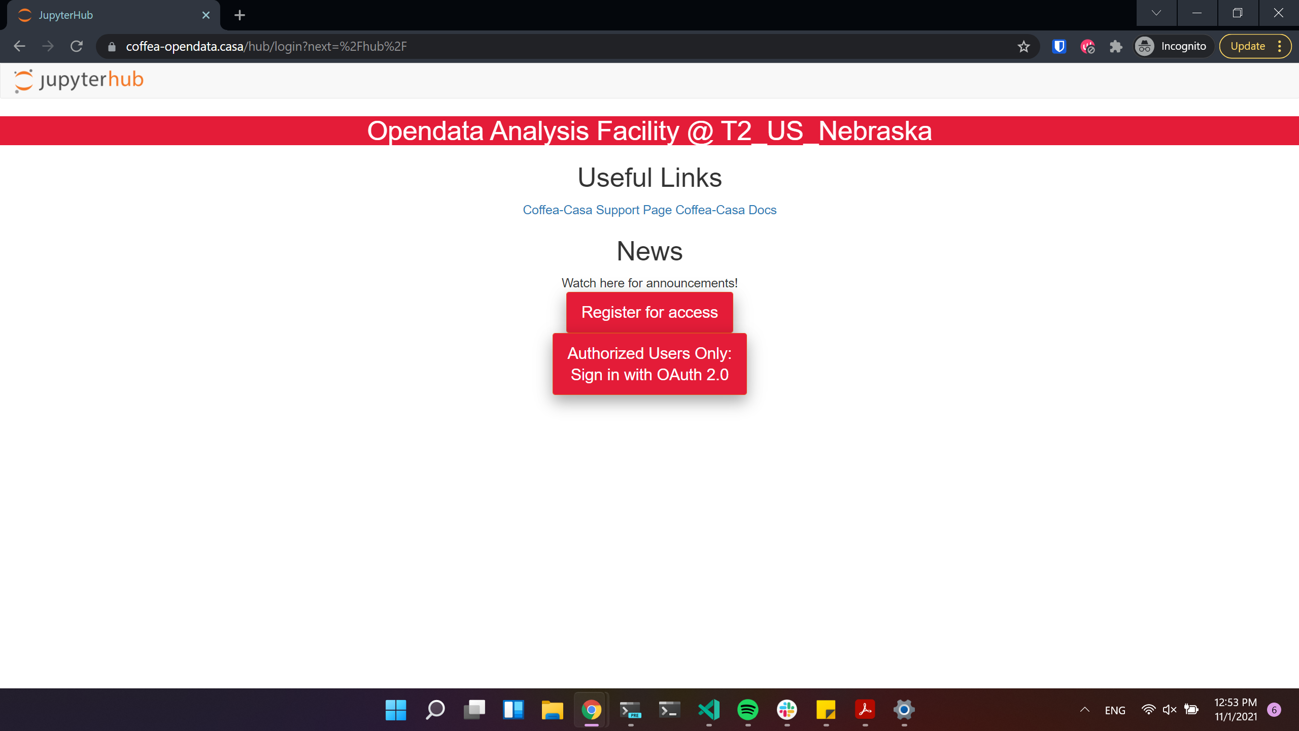
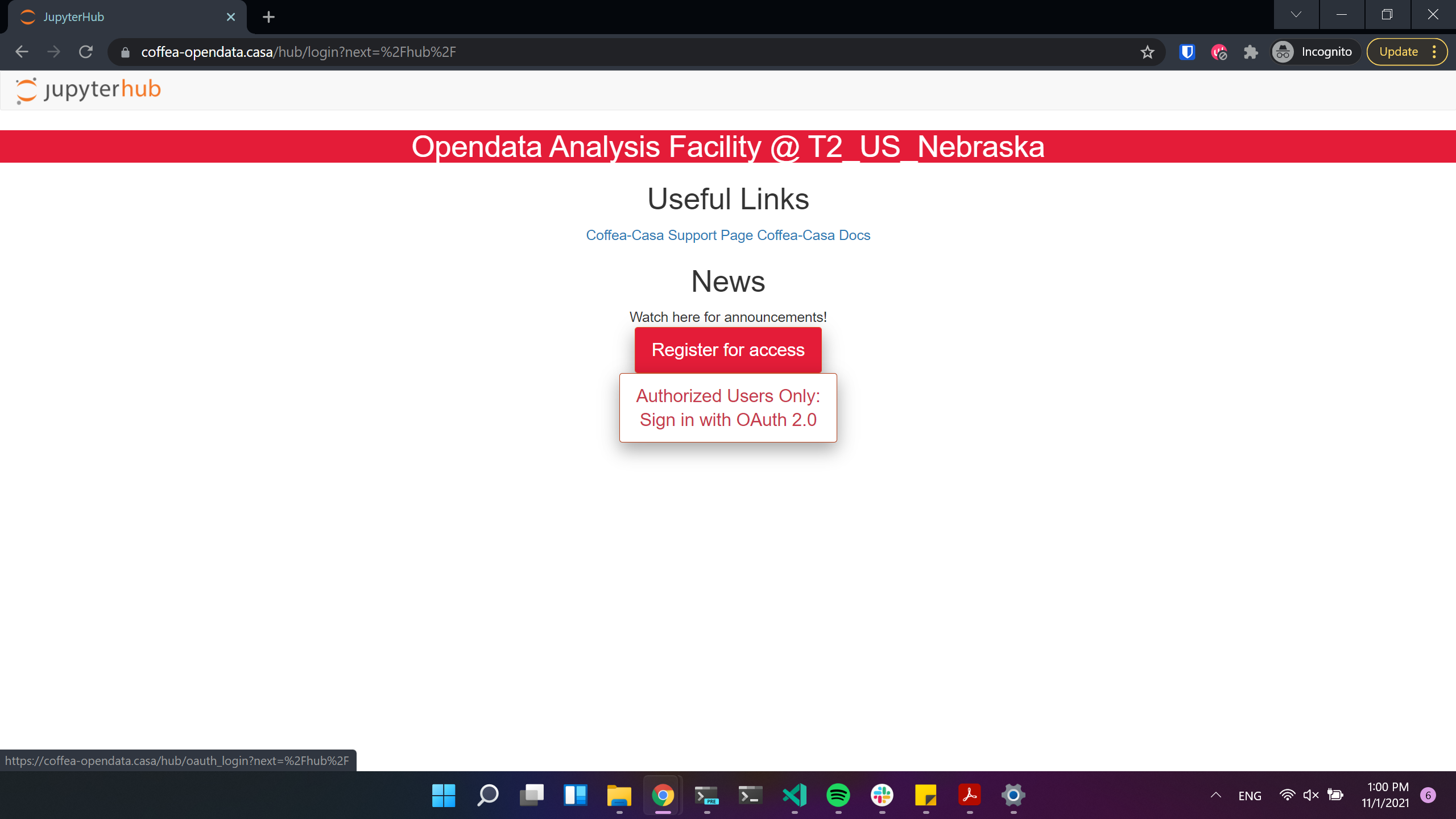
There are two access points to the Coffea-casa AF @ T2 Nebraska. The site at https://coffea-opendata.casa is for Opendata and can be accessed through any CILogon identity provider, though it will not be able to process any files that require authentication.
Important
Remember that to access this instance you need to register: click “Register for access”. (We have limited resources available and can’t provide access to everyone under CILogon).
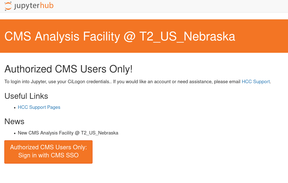
The other at https://coffea.casa is for CMS data and can be accessed through the CMS AuthZ instance; this site is capable of handling all CMS files and uses tokens for authentication.
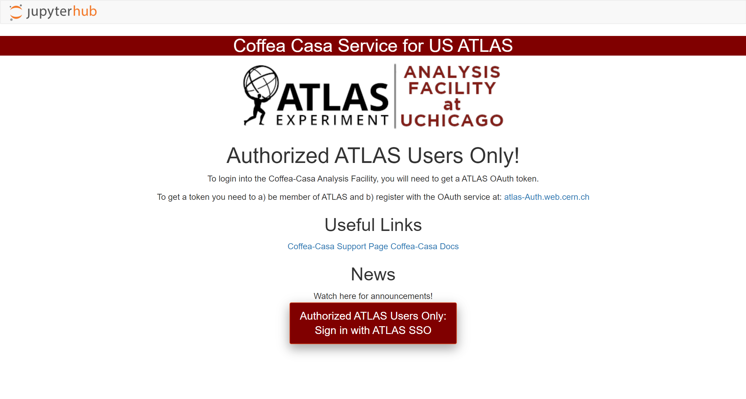
Another coffea-casa instance exists for the AF @ UChicago, which is meant to be used with ATLAS data. You can accesss it at `https://coffea.af.uchicago.edu`_.
See the appropriate section below if you need help going through the registration process for either access point.
Opendata CILogon Authentication Instance
Important
This section applies only to the Opendata Coffea-Casa instance.
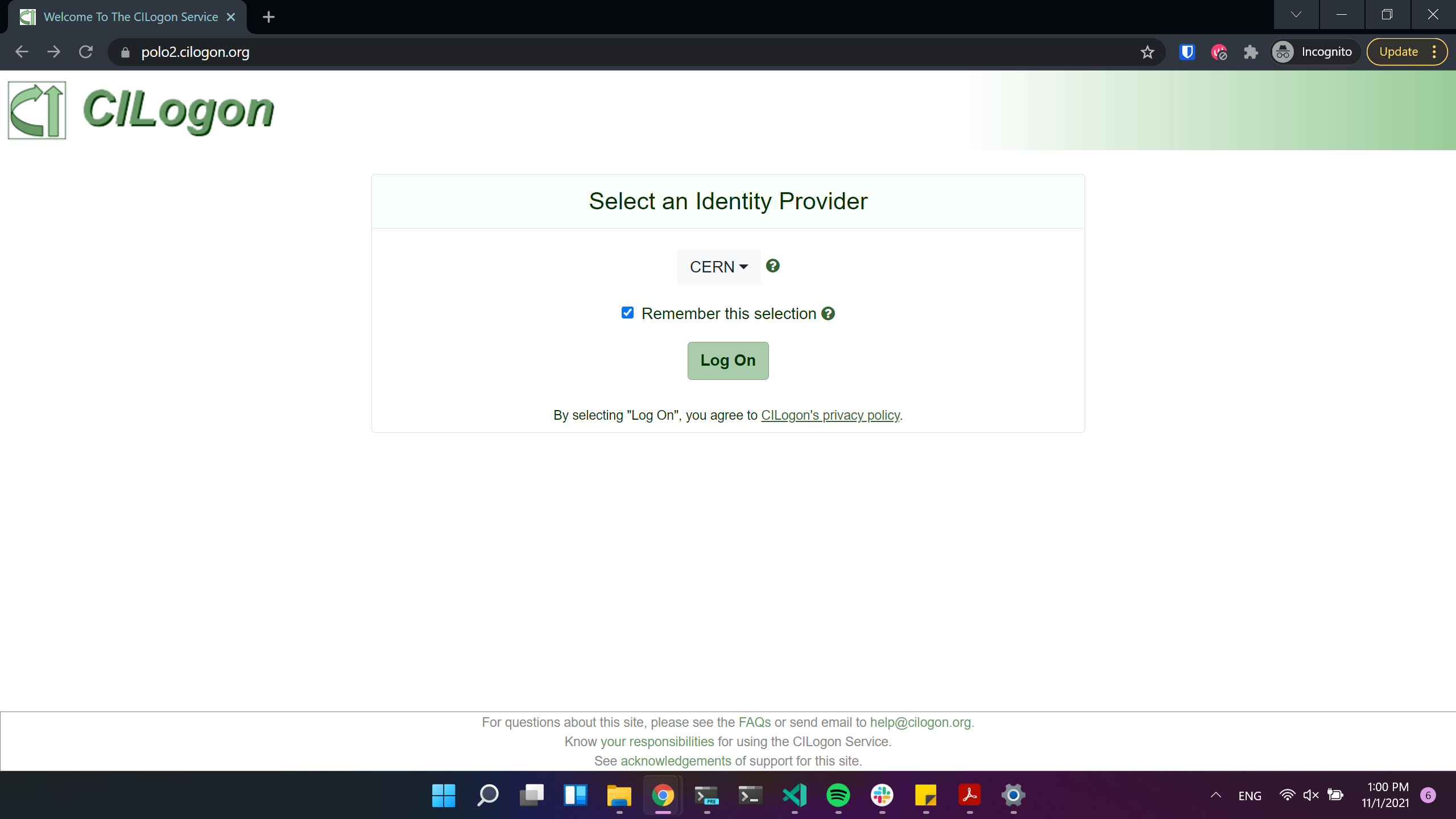
Currently Opendata Coffea-Casa supports any CILogon identity provider. Select your identity provider:
For accessing Opendata Coffea-Casa, we are offering a self-signup registration form with approval.
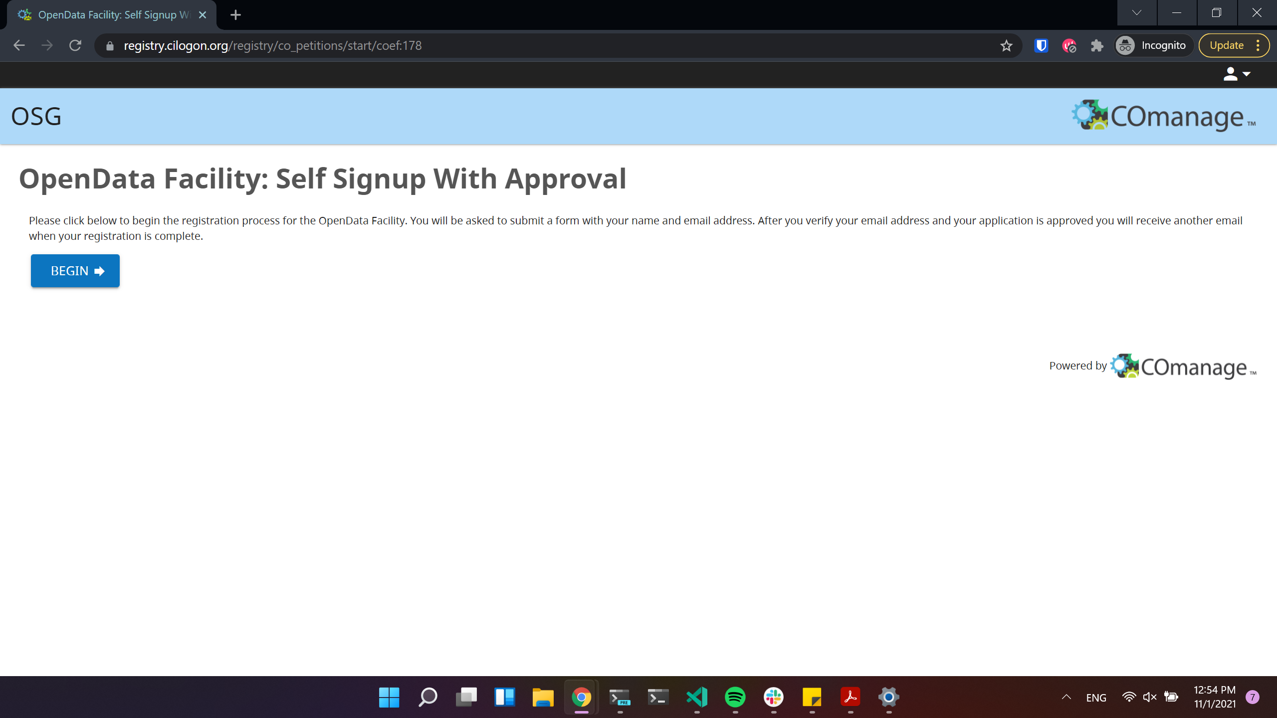
Click to proceed to the next stage:
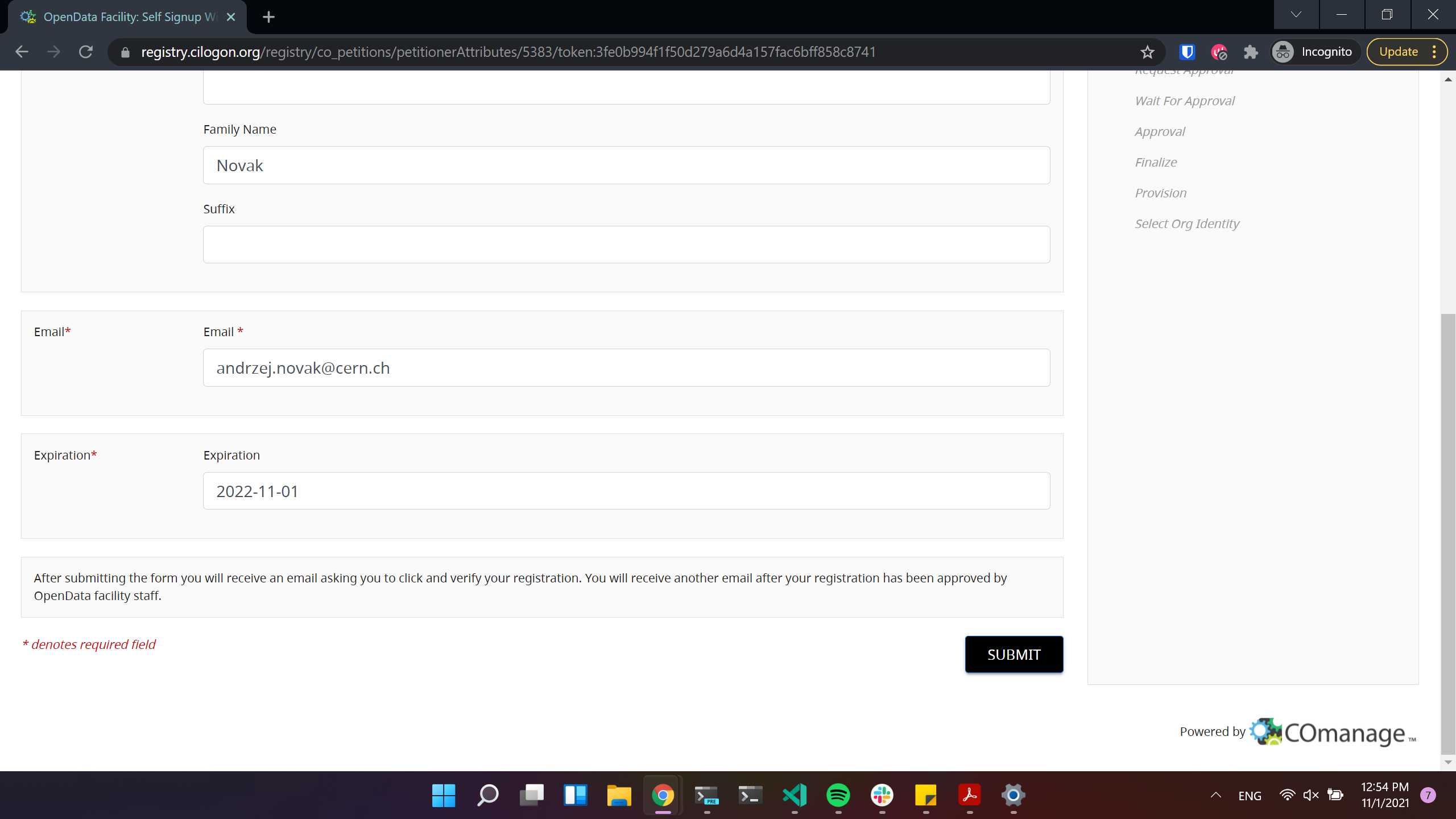
Click to proceed to the next stage:
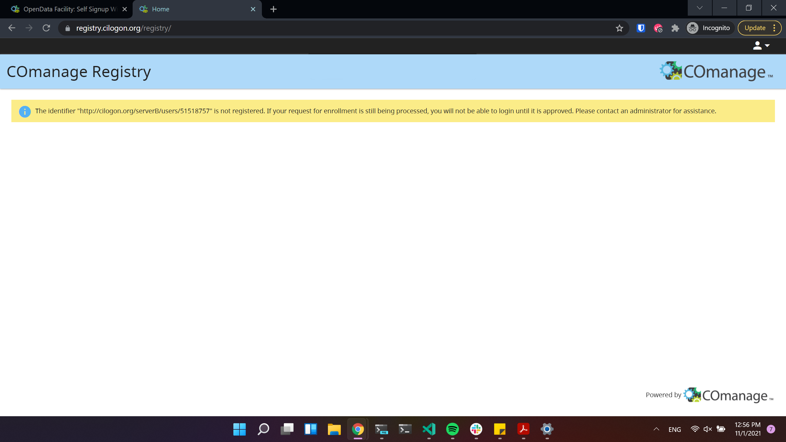
If you see the next window, it means that the registration request was sent succesfully!
Important
After this step please wait until you get approved by an administrator!
After your request is approved, you will receive an email, where you will simply need to click a link:
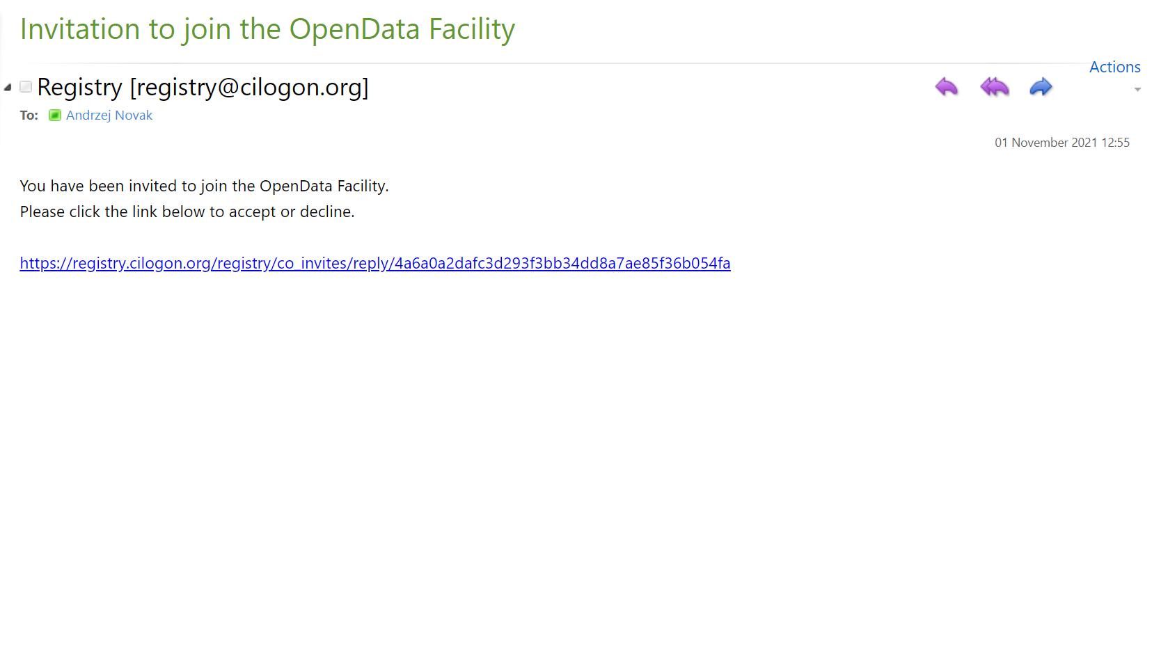
Voila! Now you can login to Opendata Coffea-Casa. Click on “Authorized Users Only: Sign in with OAuth 2.0” to do so:
CMS AuthZ Authentication Instance
Important
This section applies only to the CMS Coffea-Casa instance.
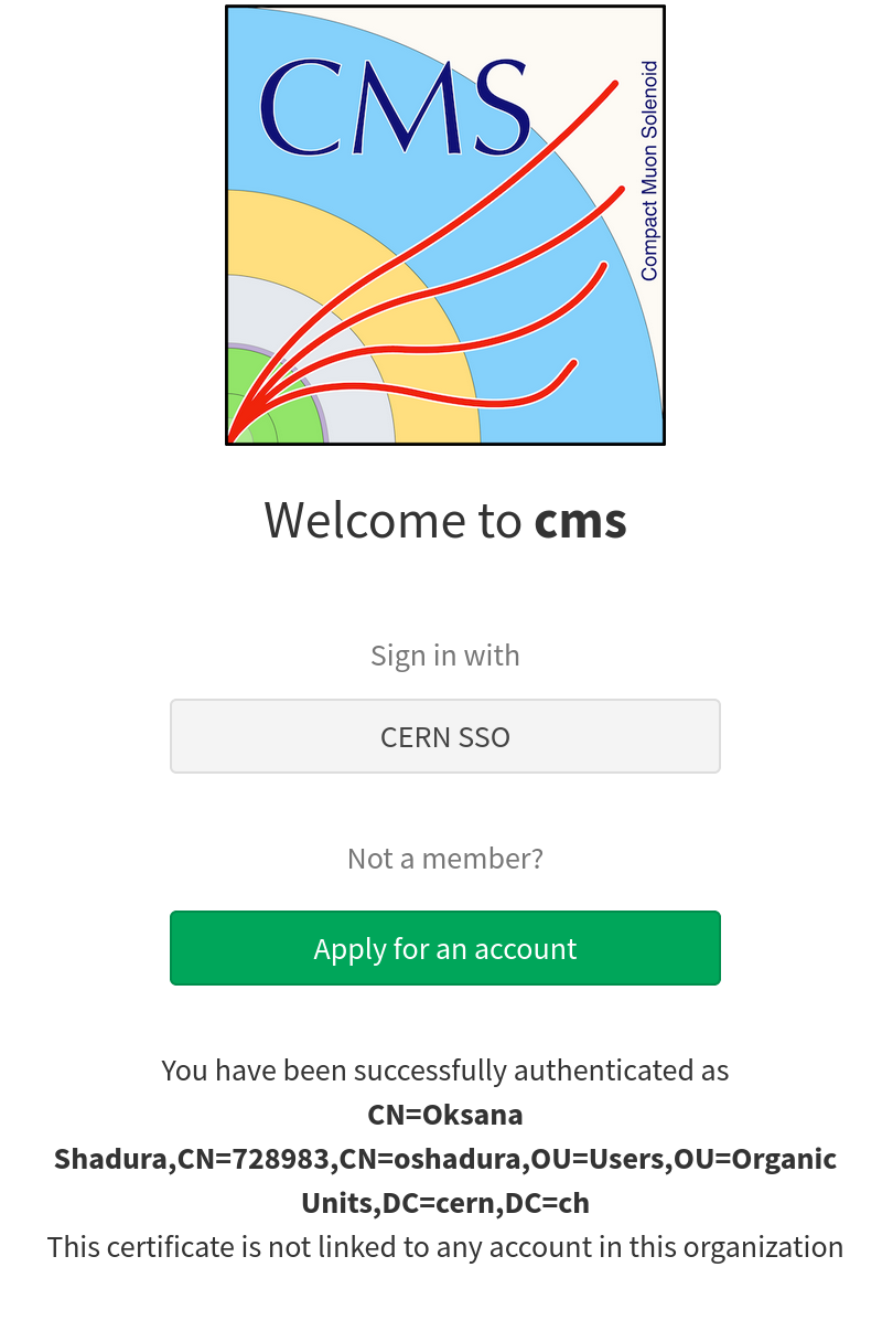
Currently Coffea-Casa Analysis Facility @ T2 Nebraska supports any member of CMS VO organisation.
To access it please sign in or sign up using Apply for an account.
ATLAS AuthZ Authentication Instance
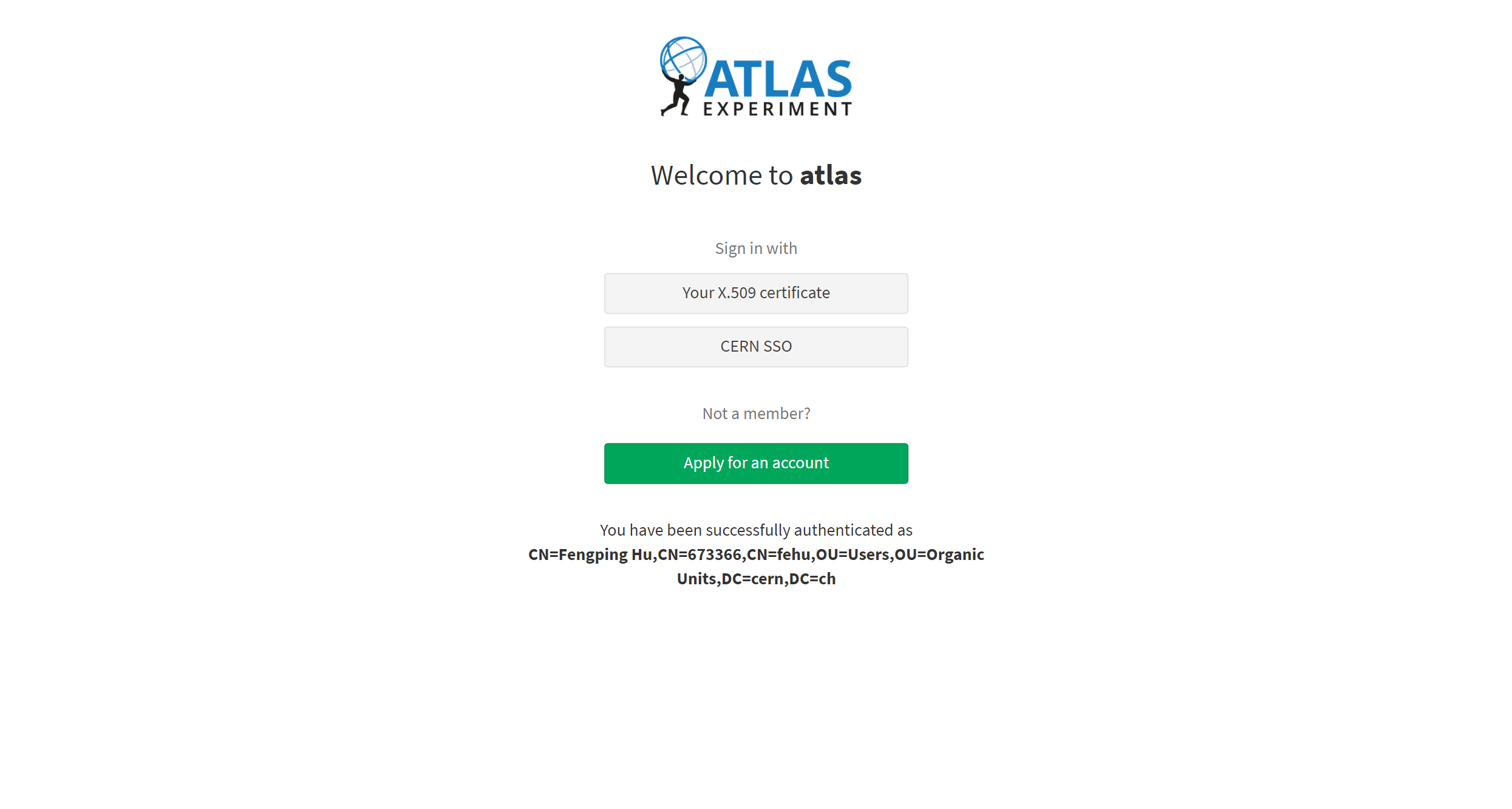
Currently Coffea-Casa Analysis Facility @ UChicago can support any member of ATLAS.
Sign in with your ATLAS CERN credential:
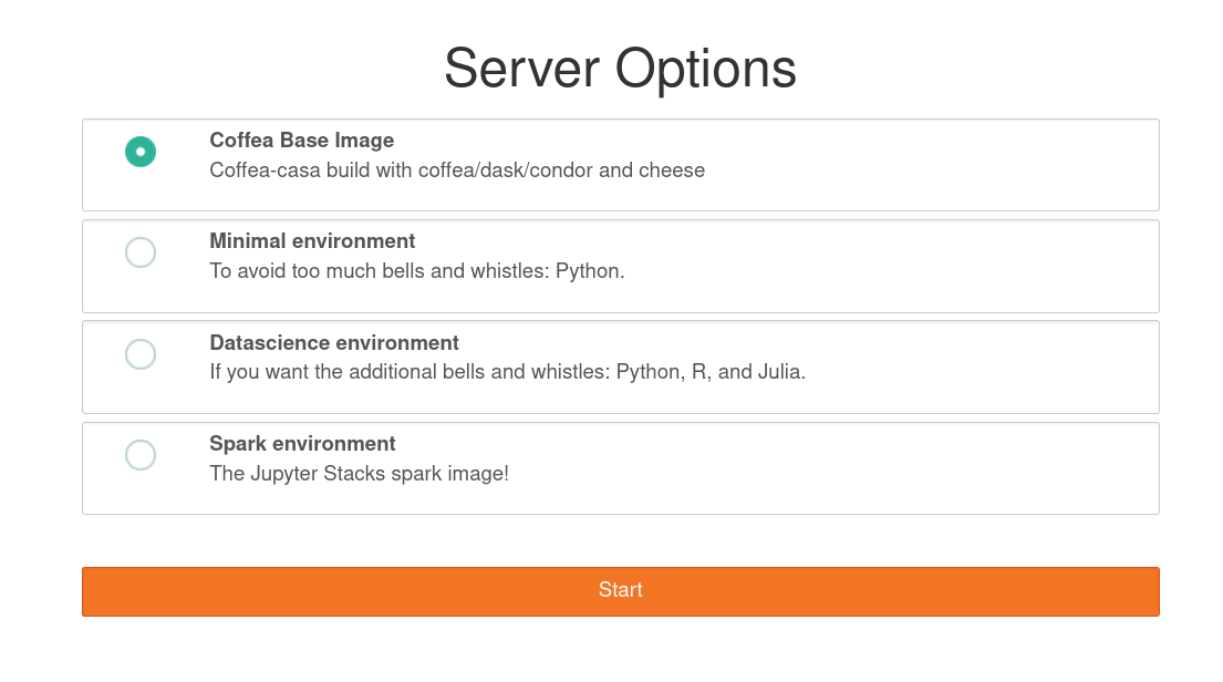
Docker Image Selection
The default image is preloaded with coffea, Dask, and HTCondor and you should select it:
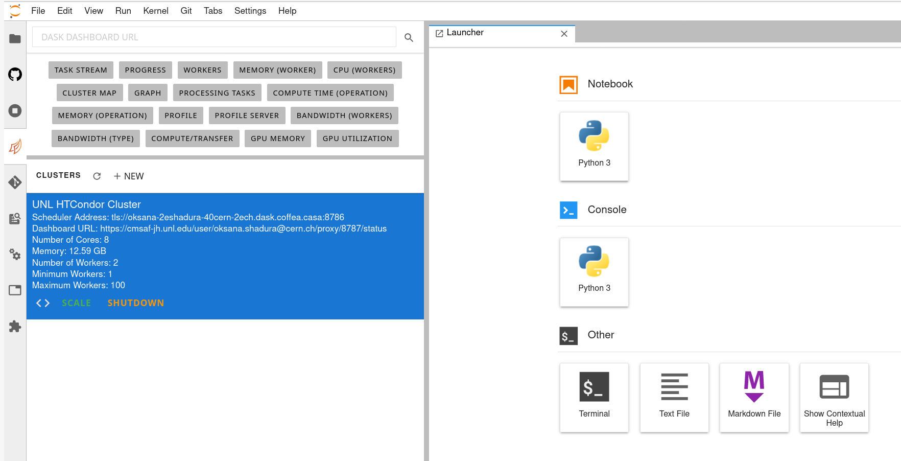
This will forward you to your own personal Jupyterhub instance running at Analysis Facility @ T2 Nebraska:
Cluster Resources in Coffea-Casa Analysis Facility @ T2 Nebraska
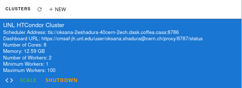
By default, the Coffea-casa Dask cluster should provide you with a scheduler and workers, which you can see by clicking on the colored Dask icon in the left sidebar.
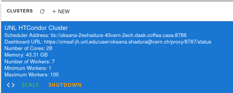
As soon as you start your computations, you will notice that available resources at the Opendata Coffea-Casa Analysis Facility @ T2 Nebraska autoscale depending on the resources available in the HTCondor pool at Nebraska Tier 2.
Cluster Hardware Specifications
The Coffea-Casa Analysis Facility @ T2 Nebraska runs on the following infrastructure:
Operating System |
AlmaLinux 9.7 |
Kubernetes Version |
1.34.5 |
GPU Resources |
2× NVIDIA L40S (available for GPU-accelerated workloads) |
Note
GPU resources (NVIDIA L40S) are available for users who require accelerated computing. Contact the facility administrators if you would like to make use of GPU nodes in your analysis.
Opening a New Console or File
There are three ways by which you can open a new tab within coffea-casa. Two are located within the File menu at the very top of the JupyterLab interface: New and New Launcher.
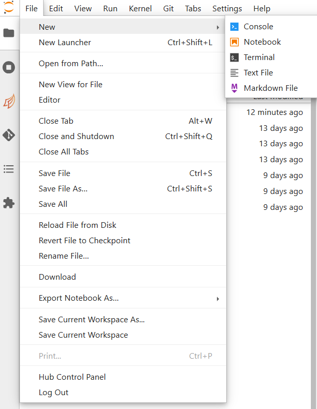
The New dropdown menu allows you to open the console or a file of a specified format directly. The New Launcher option creates a new tab with buttons that permit you to launch a console or a new file, exactly like the interface you are shown when you first open coffea-casa.
The final way is specific to the File Browser tab of the sidebar.

This behaves exactly like the New Launcher option above.
Note
Regardless of the method you use to open a new file, the file will be saved to the current directory of your File Browser.
Using Git
Cloning a repository in the Coffea-casa Analysis Facility @ T2 Nebraska is simple, though it can be a little confusing because it is spread across two tabs in the sidebar: the File Browser and the Git tabs.
In order to clone a repository, first go to the Git tab. It should look like this:
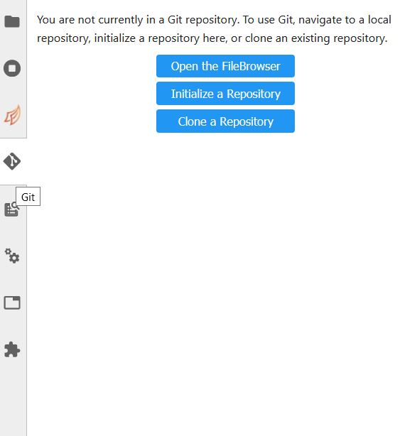
Simply click the appropriate button (initialize a repository, or clone a repository) and you’ll be hooked up to GitHub. This should then take you to the File Browser tab, which is where you can see all of the repositories you have cloned in your JupyterLab instance. The File Browser should look like this:
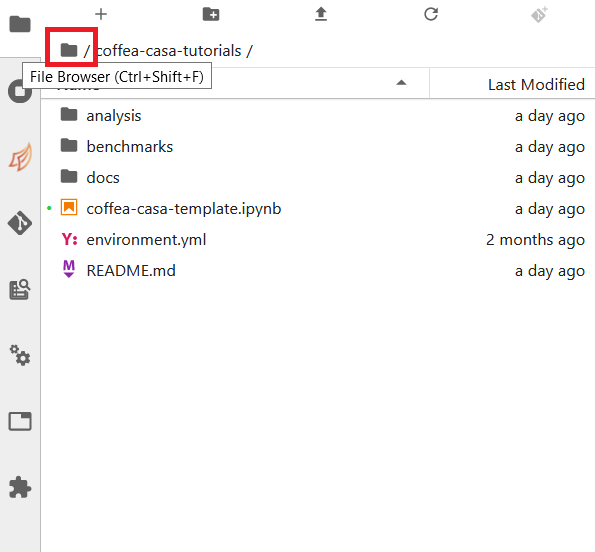
If you wish to change repositories, simply click the folder button to enter the root directory. If you are in the root directory, the Git tab will reset and allow you to clone another repository.
If you wish to commit, push, or pull from the repository you currently have active in the File Browser, then you can return to the Git tab. It should change to look like this, so long as you have a repository open in the File Browser:
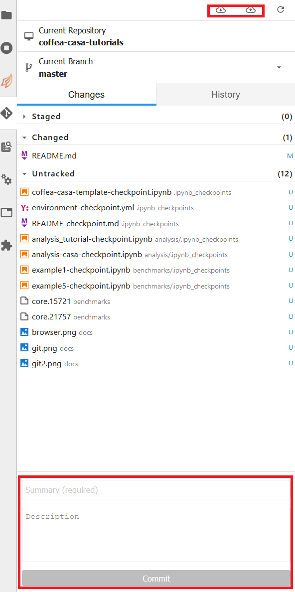
The buttons in the top right allow for pulling and pushing respectively. When you have edited files in a directory, they will show up under the Changed category, at which point you can hit the + to add them to a commit (at which point they will show up under Staged). Filling out the box at the bottom of the sidebar will file your commit, and prepare it for you to push.
Using XCache
Important
This section applies only to the CMS Coffea-Casa instance.
When we use CMS data, we generally require certificates or we will be faced with authentication errors. Coffea-casa handles the issue of certificates internally through xcache tokens so that its users do not explicitly have to import their certificates, though this dynamic requires adjustiment of the redirector portion of the path to the root file requested.
Let’s say we wish to request the file:
root://cmsxrootd.fnal.gov//store/data/Run2018A/DoubleMuon/NANOAOD/02Apr2020-v1/30000/0555868D-6B32-D249-9ED1-6B9A6AABDAF7.root
Then we would replace the cmsxrootd.fnal.gov redirector with the xcache redirector:
root://xcache//store/data/Run2018A/DoubleMuon/NANOAOD/02Apr2020-v1/30000/0555868D-6B32-D249-9ED1-6B9A6AABDAF7.root
Now, we will be able to access our data.
In addition to handling authentication, XCache will cache files so that they are able to be pulled more quickly in subsequent runs of the analysis. It should be expected, then, that the first analysis run with a new coffea-casa file will run slower than ones which follow afterwards.
ServiceX
Important
This section applies only to the ATLAS Coffea-Casa instance.
Important
This section applies only to the ATLAS Coffea-Casa instance at UChicago. The instances at T2 Nebraska are capable of handling ServiceX requests through uproot, but the feature is still at an experimental stage. Ask an administrator for more information on accessing ServiceX on the T2 Nebraska instances.
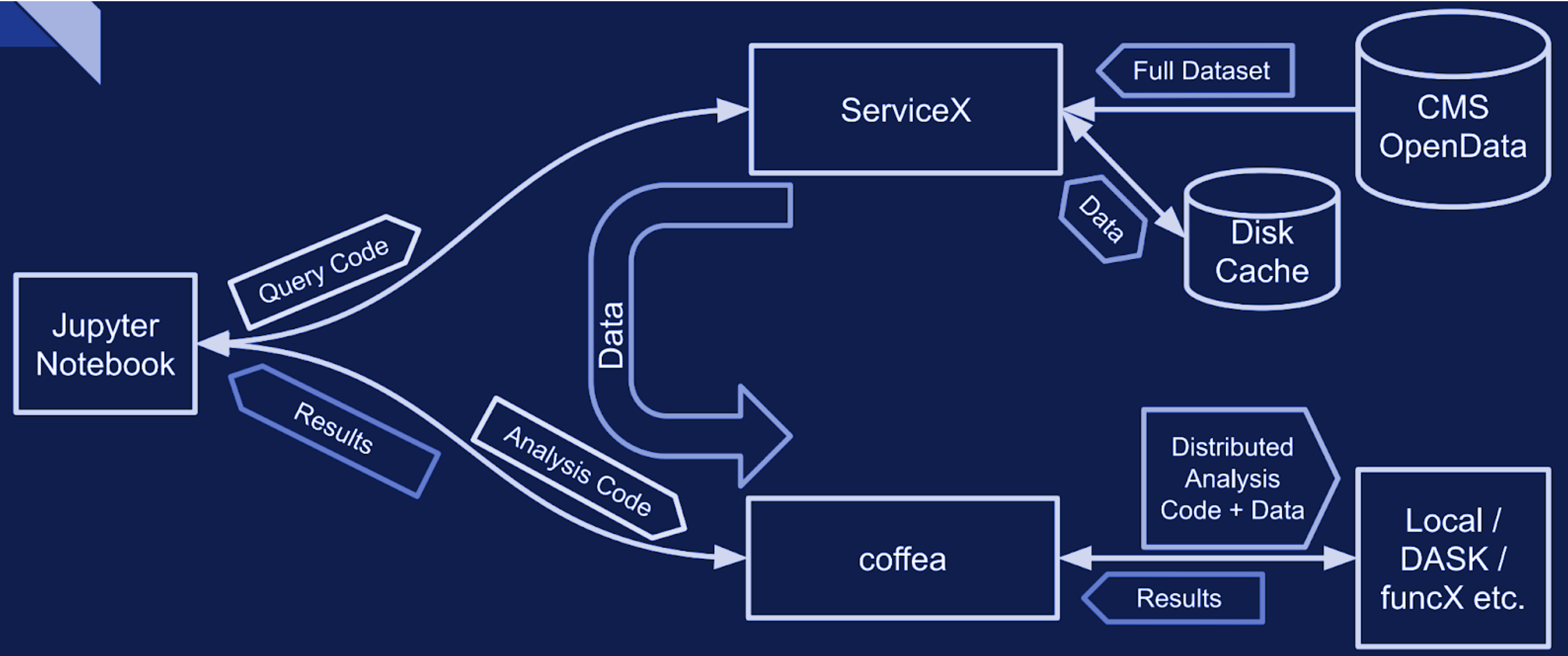
When dealing with very large datasets it is often better to do initial data filtering and augmentation using ServiceX. ServiceX transformations produce their output as an Awkward Array. The array can then be used in a regular Coffea processor. Here is a schema explaining the workflow:
There are two different UC AF-deployed ServiceX instances. The only difference between them is the type of input data they are capable of processing. Uproot processes any kind of “flat” ROOT files, while xAOD processes only Rucio registered xAOD files.
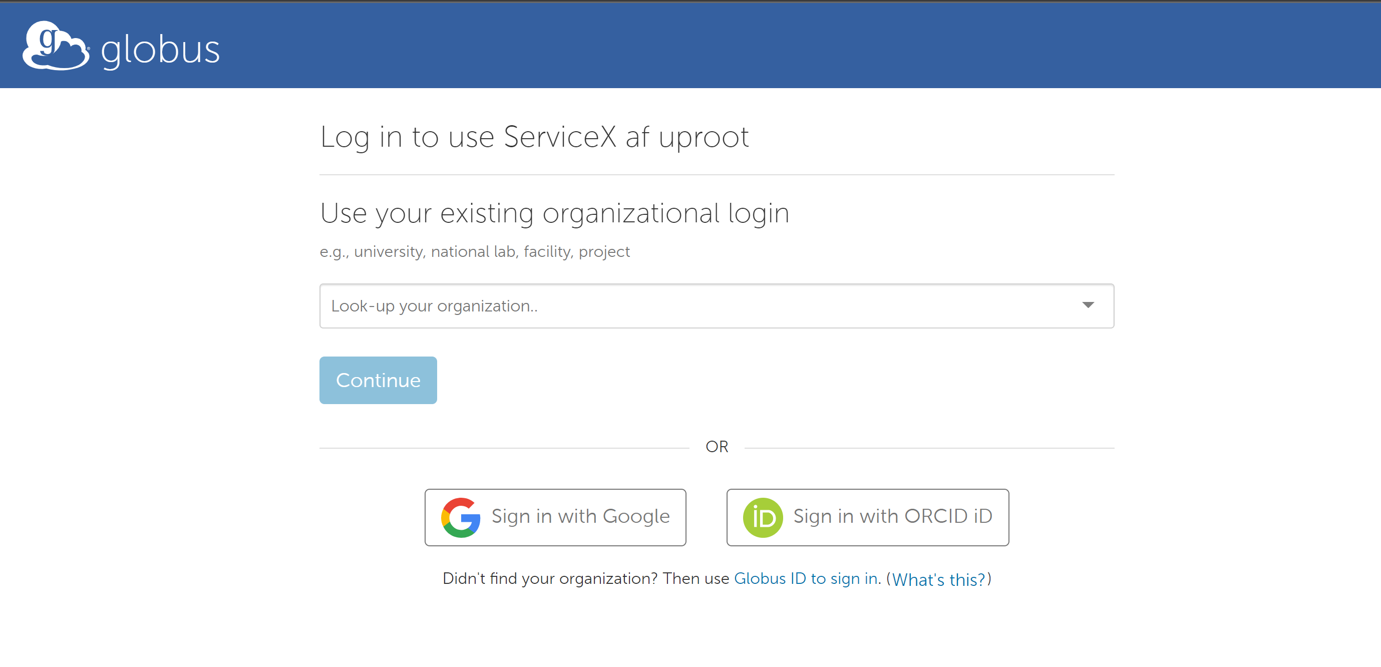
To use them one has to register and get approved. Sign in will lead you to a Globus registration page where you may choose to use an account connected to your institution:
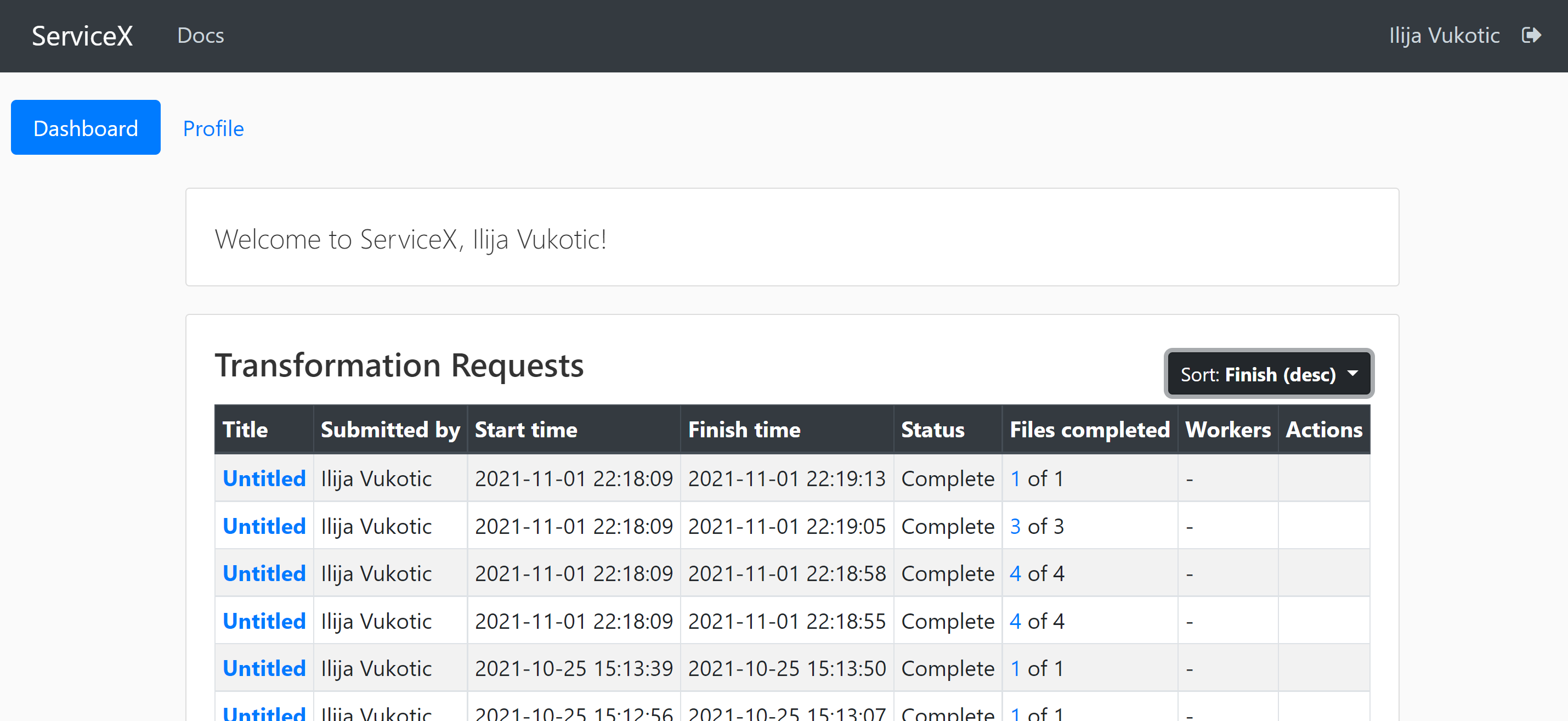
Once approved, you will be able to see the status of your requests in the dashboard:
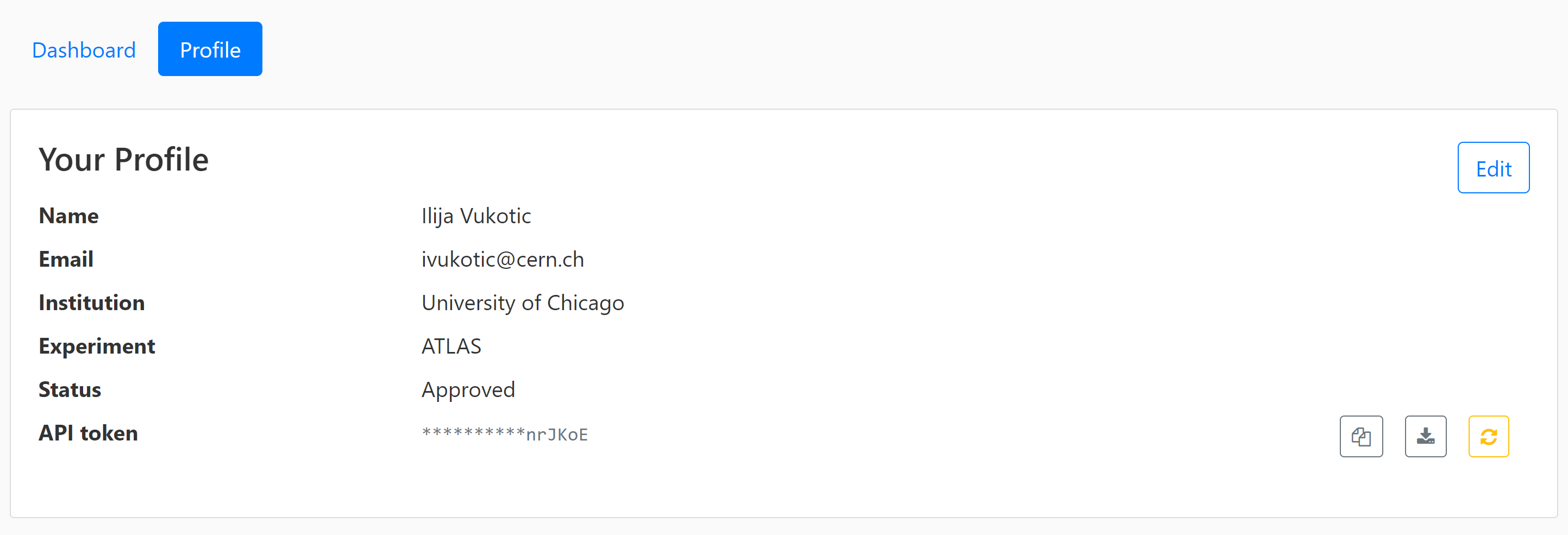
For your code to be able to authenticate your requests you need to download a servicex.yaml file, which should be placed in your working directory. The file is downloaded from your profile page:
For an example analysis using ServiceX and Coffea look here.
Opendata Example
In this example (which corresponds to ADL Benchmark 1), we’ll try to run a simple analysis example on the Coffea-Casa Analysis Facility. We will use the coffea_casa wrapper library, which allows use of pre-configured settings for HTCondor configuration and Dask scheduler/worker images.
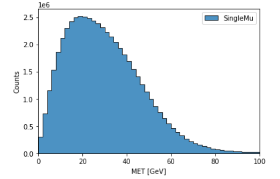
Our goal in this toy analysis is to plot the missing transverse energy (MET) of all events from a sample dataset; this data was converted from 2012 CMS Open Data (17 GB, 54 million events), and is available in public EOS (root://eospublic.cern.ch//eos/root-eos/benchmark/Run2012B_SingleMu.root).
First, we need to import the coffea libraries used in this example:
import numpy as np
%matplotlib inline
from coffea import hist
import coffea.processor as processor
import awkward as ak
from coffea.nanoevents import schemas
To select the aforementioned data in a coffea-friendly syntax, we employ a dictionary of datasets, where each dataset (key) corresponds to a list of files (values):
fileset = {'SingleMu' : ["root://eospublic.cern.ch//eos/root-eos/benchmark/Run2012B_SingleMu.root"]}
Coffea provides the coffea.processor module, where users may write their analysis code without worrying about the details of efficient parallelization, assuming that the parallelization is a trivial map-reduce operation (e.g., filling histograms and adding them together).
# This program plots an event-level variable (in this case, MET, but switching it is as easy as a dict-key change). It also demonstrates an easy use of the book-keeping cutflow tool, to keep track of the number of events processed.

# The processor class bundles our data analysis together while giving us some helpful tools.  It also leaves looping and chunks to the framework instead of us.
class Processor(processor.ProcessorABC):
    def __init__(self):
        # Bins and categories for the histogram are defined here. For format, see https://coffeateam.github.io/coffea/stubs/coffea.hist.hist_tools.Hist.html && https://coffeateam.github.io/coffea/stubs/coffea.hist.hist_tools.Bin.html
        dataset_axis = hist.Cat("dataset", "")
        MET_axis = hist.Bin("MET", "MET [GeV]", 50, 0, 100)

        # The accumulator keeps our data chunks together for histogramming. It also gives us cutflow, which can be used to keep track of data.
        self._accumulator = processor.dict_accumulator({
            'MET': hist.Hist("Counts", dataset_axis, MET_axis),
            'cutflow': processor.defaultdict_accumulator(int)
        })

    @property
    def accumulator(self):
        return self._accumulator

    def process(self, events):
        output = self.accumulator.identity()

        # This is where we do our actual analysis. The dataset has columns similar to the TTree's; events.columns can tell you them, or events.[object].columns for deeper depth.
        dataset = events.metadata["dataset"]
        MET = events.MET.pt

        # We can define a new key for cutflow (in this case 'all events'). Then we can put values into it. We need += because it's per-chunk (demonstrated below)
        output['cutflow']['all events'] += ak.size(MET)
        output['cutflow']['number of chunks'] += 1

        # This fills our histogram once our data is collected. The hist key ('MET=') will be defined in the bin in __init__.
        output['MET'].fill(dataset=dataset, MET=MET)
        return output

    def postprocess(self, accumulator):
        return accumulator
With our data in our fileset variable and our processor ready to go, we simply need to connect to the Dask Labextention-powered cluster available within the Coffea-Casa Analysis Facility @ T2 Nebraska. This can be done by dragging the scheduler into the notebook, or by manually typing the following:
from dask.distributed import Client
client = Client("tls://localhost:8786")
Then we bundle everything up to run our job, making use of the Dask executor. We must point it to our client as defined above. In the Runner, we specify that we want to make use of the NanoAODSchema (as our input file is a NanoAOD).
executor = processor.DaskExecutor(client=client)
run = processor.Runner(executor=executor,
                        schema=schemas.NanoAODSchema,
                        savemetrics=True
                      )

output, metrics = run(fileset, "Events", processor_instance=Processor())
The final step is to generates a 1D histogram from the data output to the ‘MET’ key. fill_opts are optional arguments to fill the graph (default is a line).
hist.plot1d(output['MET'], overlay='dataset', fill_opts={'edgecolor': (0,0,0,0.3), 'alpha': 0.8})
As a result you should see the following plot:
CMS Example
Important
This section applies only to the CMS Coffea-Casa instance.
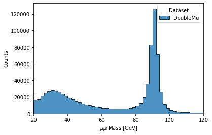
Now we will try to run a short example, using CMS data, which corresponds to plotting the dimuon Z-peak. We use dimuon data which consists of ~3 million events at ~2.7 GB which belongs to the /DoubleMuon/Run2018A-02Apr2020-v1/NANOAOD dataset.
We import some common coffea libraries used in this example:
import numpy as np
from coffea import hist
from coffea.analysis_objects import JaggedCandidateArray
import coffea.processor as processor
%matplotlib inline
To select the aforementioned data in a coffea-friendly syntax, we employ a dictionary of datasets, where each dataset (key) corresponds to a list of files (values):
fileset = {'DoubleMu' : ['root://xcache//store/data/Run2018A/DoubleMuon/NANOAOD/02Apr2020-v1/30000/0555868D-6B32-D249-9ED1-6B9A6AABDAF7.root',
                        'root://xcache//store/data/Run2018A/DoubleMuon/NANOAOD/02Apr2020-v1/30000/07796DC0-9F65-F940-AAD1-FE82262B4B03.root',
                        'root://xcache//store/data/Run2018A/DoubleMuon/NANOAOD/02Apr2020-v1/30000/09BED5A5-E6CC-AC4E-9344-B60B3A186CFA.root']}
Coffea provides the coffea.processor module, where users may write their analysis code without worrying about the details of efficient parallelization, assuming that the parallelization is a trivial map-reduce operation (e.g., filling histograms and adding them together).
class Processor(processor.ProcessorABC):
    def __init__(self):
        dataset_axis = hist.Cat("dataset", "Dataset")
        dimu_mass_axis = hist.Bin("dimu_mass", "$\mu\mu$ Mass [GeV]", 50, 20, 120)

        self._accumulator = processor.dict_accumulator({
            'dimu_mass': hist.Hist("Counts", dataset_axis, dimu_mass_axis),
        })

    @property
    def accumulator(self):
        return self._accumulator

    def process(self, events):
        output = self.accumulator.identity()

        dataset = events.metadata["dataset"]

        mu = events.Muon
        # Select events with 2 muons whose charges cancel out (Zs are charge-neutral).
        dimu_neutral = mu[(ak.num(mu) == 2) & (ak.sum(mu.charge, axis=1) == 0)]
        # Add together muon pair p4's, find dimuon mass.
        dimu_mass = (dimu_neutral[:, 0] + dimu_neutral[:, 1]).mass
        # Plot dimuon mass.
        output['dimu_mass'].fill(dataset=dataset, dimu_mass=dimu_mass)
        return output

    def postprocess(self, accumulator):
        return accumulator
With our data in our fileset variable and our processor ready to go, we simply need to connect to the Dask Labextention-powered cluster available within the Coffea-Casa Analysis Facility @ T2 Nebraska. This can be done by dragging the scheduler into the notebook, or by manually typing the following:
from dask.distributed import Client
client = Client("tls://localhost:8786")
Then we bundle everything up to run our job, making use of the Dask executor. To do this, we must point to a client within executor_args.
executor = processor.DaskExecutor(client=client)
run = processor.Runner(executor=executor,
                        schema=schemas.NanoAODSchema,
                      )

output = run(fileset, "Events", processor_instance=Processor())
The final step is to generates a 1D histogram from the data output to the ‘MET’ key. fill_opts are optional arguments to fill the graph (default is a line).
hist.plot1d(output['dimu_mass'], overlay='dataset', fill_opts={'edgecolor': (0,0,0,0.3), 'alpha': 0.8})
As a result you should see the following plot:
ATLAS Examples
Important
This section applies only to the ATLAS Coffea-Casa instance.
The notebooks about columnar data analysis with DAOD_PHYSLITE `here<https://github.com/nikoladze/agc-tools-workshop-2021-physlite>`_ may be useful as a reference.